Ennova, AI and CFD

The application of AI (Artificial Intelligence) to CFD (Computational Fluid Dynamics) is the latest in a long history of advancements that have decreased the time it takes to go from design to prediction. As the cost and time to calculate performance from design gets smaller and smaller, we get closer and closer to the vision of being able to automatically optimize or even automate product design.

Neural networks promise to be the the next quantum leap in CFD performance. AI-based CFD will necessarily require highly automatic mesh generation tools in the creation of the synthetic databases required to train the neural networks used in AI-based CFD. Additionally, if the AI is trained as CFD workalike (surrogate) for arbitrary geometries, very high speed mesh generation will be required not only in the training phase but also in the inference phase of AI-based CFD.

A Short History

Although AI-based CFD will be a quantum improvement in the speed of CFD it will not be the first. What follows is a quick history of technological breakthroughs that have brought CFD to where it is today. If you want to skip ahead to the AI part, click here

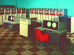
We can trace the advancement in the speed of CFD starting in the 1960's when the first CFD codes ran on early scientific computers such as the CDC 6600. Advancements came from more advanced computer architectures, smaller and faster electronics and improvements to software algorithms. AI-based CFD, like other advancements, is enabled by a new hardware architecture, the GPU, and a new software approach, machine learning, specifically neural networks.

Vector Processors

The first advancements in computer architecture came with Vector Processors. The key observation that makes vector processors a signficant improvement over a scalar processor, is that tens or hundreds or thousands of operations that a computer must perform are so similar to each other that much of the control logic is not needed and more of the hardware can be devoted to the actual work of the computer: multiplying floating point numbers. On a general purpose computer, on a generic piece of software, each executed instruction might be completely different than then next, with different data types, coming from unrelated parts of memory and being executed based on conditions specific to that instruction. In that case, a large portion of the computer hardware must be dedicated to decoding instructions, branching on conditionals and managing the reading and writing of data. This would be single instruction, single data (SISD).

For CFD and other scientific calculations, it was noticed that tens or hundreds of executed instructions were just the same operation repeated on consecutive locations in memory. Running on a scalar computer, the CPU would decode the same instruction hundreds of times, evaluate conditionals hundreds of times, issue fetch operations hundreds of times, and also issue store operations hundreds of times. The idea was to decode the vector instruction once, tell the memory system of load a whole series of data locations once, pipeline the actual operation through the functional unit and then store the data back to memory in regular pattern. This is called single instruction, multiple data (SIMD).

Algorithmic Improvements

Simultaneous to this, programmers were improving the software that was running on this improved hardware, by using Successive Over-Relaxation (SOR), Multigrid and other methods.

Parallel Processing

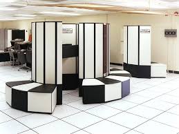
The next hardware leap came from parallel processing, where a single computer comprised more than a single independent CPU. Early supercomputers featured several astronomically priced vector CPU's linked into a single system that could divide a large CFD problem into first 4 then 8 and then 16 separate problems that could be mostly independently solved with separate pieces updating each other from time to time.

Clusters

By the early 90's, inexpensive comodity chips used in personal computers started to have processing power that approached that of the CPU's of specialty supercomputers. By linking together hundreds of inexpensive systems, researchers could build a virtual supercomputer for the fraction of the price.

Multi-core CPU's

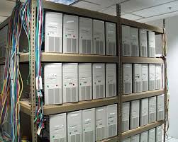
By the early 2000's, commodity chips were being produced with multiple CPU's. All of these advancements were layered on top of each other and the performance gains were multiplied. A linux cluster could be built from hundreds or thousands of "nodes". A node is essentially a standalone computer about the size of a pizza box, that has it's own power suppply, several CPU's, its own memory and networking hardware. Each CPU was really a chip containing several "cores", each "core" was really what used to called a CPU, a piece of hardware with its own program counter and instruction decode logic and functional units such as floating point adders and multipliers.

Inside of each "core" the functional units were pipelined, meaning at each clock cycle a different operand worked its way partially through the functional unit. So at any given time the floating point multiplier was processing portions of several instructions. In this way more and more of the electronics were being used all of the time.

GPU's

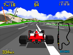
The next revolution in computation, came from "left field" so to speak. While one group of users was concerned with solving systems of millions of equations for scientific and industrial reasons (grown adults with paying jobs), a completely different group of users (mostly teenage boys) were playing video games with more and more realistic graphics. The compuational power required to render a screen for a computer game is actually on the same scale as needed for a cutting edge CFD calculation. But in the early days, the graphics cards were custom built to do only computer graphics and could be optimized to do just that task. They were not programmable in the traditional sense.

A GPU worked by having a large array of identical relatively slow processors, each of which was only responsible for rendering a small portion of the screen.

GPGPU's

As more and more sophisticated graphics effects were being implemented, it became harder and harder to implement that in "burned in" graphics chips. An new kind of graphics chip was invented: the general purpose graphics processing unit (GPGPU). There is still the array of many relatively lower speed processors all working in lockstep, but the calculations they were performing were programmable. It was more like an array of functional units than an array of CPU's or cores. But now this array of functional units was programmable. Now the GPU controller could say to its array of processors "each of you hundreds of units: read a data location, perform this operation and then store". Suddenly a single GPU behaved like a CPU but with hundreds of times the power, as long as it had hundreds of identical tasks to perform.

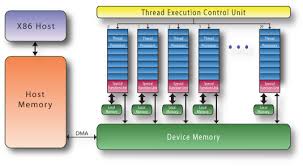
A GPU cannot do what a regular CPU core can do hundreds of times faster, unless the tasks is repetive in a very restrictive way. But for computer graphics it worked. And people doing matrix operations quickly realized that it would also work for them as well.

CFD on GPU's

Because GPU's are programmed in a completely different paradigm than either parallel computers or serial computers, a CFD code typically needs to be completely re-written in order to take advantage of GPU's. When this is done, the speedups can be dramatic. For existing code that are adapted to GPU's the speedup can be from 10 x to 100 x. A few native built GPU based CFD codes exist today such as LEO from ADS, Flow360 from Flexcompute or Luminary Cloud's GPU based solver. Those GPU native codes tend to have more dramatic speed advantages. Most existing solvers are also incorporating GPU technology into their code but the coverage is spotty.

Neural Networks

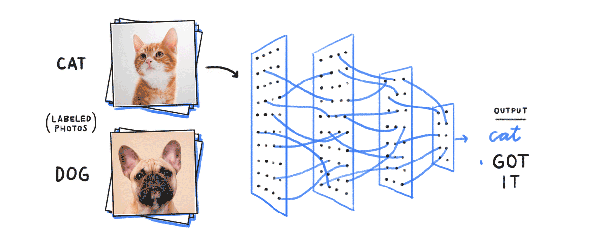
At the same time that CFD solver programmers were taking advantage of GPU's, another completely independent group of people were taking advantage of them as well. Researchers in AI had long struggled with making their neural networks do anything meaningful. A neural network works as follows. Suppose you want to create a program that can tell the difference between pictures of dogs and cats. If the pictures were black and white with a grey scale value at each pixel, the set of pixels would be a set of N input floating point values: 0 for black, 1 for white, .5 for medium grey and so on. Each pixel would be connected to the inputs of many neurons and each connection would have a weight.

In our brains, if the sum of the input values times their weights pass a threshhold the neuron would fire. In a computer this step function is replaced by an activation function that is essentially a slightly smoothed out version of the step function.

We know that this is the mechanism in our brains and we can tell the difference between images of dogs and cats, so in theory there must be a man-made neural network we can implement on a computer that will do the same thing. Of course, there nearly 100 billion neurons in a human brain and we don't know how they are interconnected. The plan for AI was to create a multi-level network of neurons, and increase the number of levels and number of neurons on each level until some useful result emerged. Of course, we don't know the weights and we don't want to figure them out "by hand". We want the determination of the weights to be done by the computer. This is the machine learning part.

The process of determining the weights is called "training" and it works like this. We start by labelling "by hand" all the images as dogs or cats. The pictures along with the correct answer "dog" or "cat" is our training data. We start with some initial set of weights and run all the images through the neural network and we get a measure of how well this neural network performs: the percentage of correct answers. This is called the loss function or objective function Now we perform the key step. We need to adjust the all of the weights so that the loss function is optimized. For purposes of explanation, let's consider how the loss function can be improved by changing a single weight. If we change a single weight, the loss function may get better, worse or remain unchanged. This is the partial derivative of the loss function with respect to a single weight. The combination of all of the partial derivatives is the gradient of the loss function. Calculating the partial derivative efficiently through the network is called backpropagation. We need the activation function to be smooth and not step-like so that the loss function is differentiable.

The gradient is the combination of weight adjustments that improves the loss function the quickest. The algorithm that uses the gradient, makes a small step in the direction of the gradient and then re-evaluates the loss function (or objective function) is call gradient descent. There are variants of gradient descent such as stochiastic gradient descent.

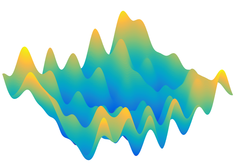
We are in an N dimensional space, where N is the number of neuron weights and we have a smooth scalar function, the performance that we want to optimize. If we only had two weights to fiddle with, the space we would have to explore might look like the above picture, where we have to wander around until we find the highest point. Computational scientists have studied this problem for years and it is the well known optimization problem. The advent of GPU's made available the kind of massive and cheap computational power needed to solve the optimization problem of finding the neural network weights, and suddenly computers could tell dogs from cats understand natural language and answer any question you might have.

While neural networks take a tremendous amout of time to train, they take only incredibly small amount of time to execute. In fact, the training of a neural network amounts of running on each item of your dataset through your neural network, rating the performance of your neural network, adjusting the weights and then iterating again. So the computation needed is = (the number of items in your dataset) x ( number of iterations) x (cost of one inference). If you dataset is 25,000 images and you have to iterate 100,000 times, that's 2,500,000,000 (2.5 billion) evalations of the neural network. So executing a neural network (performing an inference) will be many orders of magnitidue faster than training it.

CFD, AI and Neural Networks

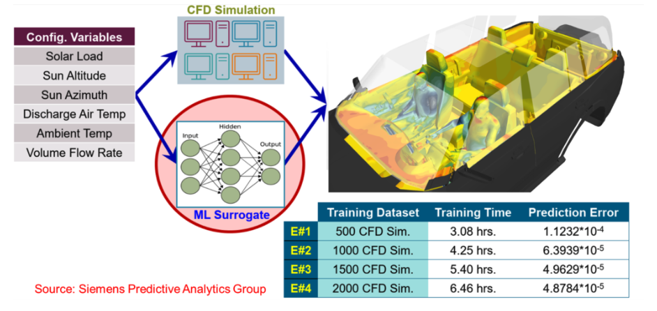
Since running a CFD simulation is quite time consuming (even using GPU's) it now becomes interesting to explore if training neural networks to predict fluid flow is feasible. We should now make the distiction between two different ways to use AI in conjuction witih CFD. One is to augment CFD by incorporating AI into turbulence models, but generally keeping the overal framework of solving a system of non-linear physics equations. The second is to replace CFD entirely with a neural network and create a surrogate model.

In the augmentation model we are applying AI locally on the mesh and selecting the parameters of a turbulence model based local physical conditions. This neural network is a map from however many numbers describe the local physics at a point in space, to the appropriate parameters of a turbulence model. So this might be a map from 10 or twenty numbers to the half a dozen parameters of turbulence model. The training data for this could be real experiments or synthetic data from more sophisticated CFD models such as LES that model turbulence directly. Hybrid turbulence modeling is an active area of research.

One would expect that the augmentation model could have a very broad application. In fact, is has to, since it must represent what is happening to turbulence in different parts of the model where the flow rate is going from 0 to supersonic and from laminar to turbulent. This AI model would be trained once and re-used millions of times even on a single CFD run, and would be used on a wide variety of CFD runs.

In the surrogate model, we are replacing the whole framework of solving a large system of non-linear equations with a neural network. For both the input and the output of the neural network we have some choices. For the input we could have a handful of parameters, such as wing chord, span and thickness and fuselage legnth and diameter. On the other extreme, we could have the input to the neural network be a generic mesh of a aircraft and wind tunnel, together with boundary conditions.

Similarly on the output side we could ask the neural network to predict just two numbers, lift and drag. Or we could ask it to predict the pressure distribution over the entire aircraft.

All pairs of of these input and output data sizes are possible but some make more sense than others. For instance, going from a handful of design parameters to a small number of performance metrics is going to tbe require the smallest amount of training data and will be situation that mimics actual CFD the best. Going from generic mesh input to full pressure distribution is really a research proposition at this point and will require perhaps hundreds of thousands of CFD runs as training data will likely only be acurate over a small range of geometric changes to the input. In this case the neural network is supposed to learn how fluid works on a large scale rather than just in the neighborhood of a single mesh node or cell.

Let's drill down on the second case where we are trying to make a surrogate model for a CFD problem presented as a generic mesh. A mesh with 100,000 vertices has to be considered at least a 300,000 dimensional space. If we include the mesh topology it is only worse. If we are trying to map out CFD behaviour inside a ball with hypercube with First, we would have to decide on a fairly restricted space to explore, perhaps airflow over an aircraft where we would vary the geometry of the airfoil and perhaps the velocity or temperature or pressure. If we are only interested in an optimal design at a specific airspeed, temperature and pressure; it would probably be best not to vary those parameters. After deciding the space to expore, we would need to generate thousands or tens of thousands of CFD results in that space. If our final neural network is going to take a handful of design parameters as an input, tens of thousands of CFD results may be sufficient. If our neural network is going to take an arbitrary surface mesh as an input, the training data may require hundreds of thousands or millions of CFD runs. In either case, these results are completely independent of each other (from a compuational standpoint) and could thus be run in parallel on potentailly completely independent computers. After computing this dataset, we would use it train a neural network.

Here we have choice about what our AI-CFD will look like. We can make the input to the neural net be simply the design variables that we varied to produce the different cases and make the output the parameters of interest. For instance, we could make the design variables be the wing chord, span and thickness and we could measure the lift and drag.

On the other hand, we could make the input to the neural net be the mesh itself. If the mesh is the input to the neural net then it comprises hundreds of thousands of variables, rather than just the few that we varied to produce the training set.

The input to neural network would be just the mesh and the boundary conditions at each node or face. In theory, we could make the volume mesh part of the input, however, if we are only interested in the pressures on the surface of the aircraft (to compute lift and drag), we don't really need it. And besides, in the real world as well as in the perfect mathematical continuum that we are trying to model, there exists a solution independent of the discretization. That's the whole point of mesh convergence studies: trying to find the volume solution that a series of more and more dense meshes converge to.

The output we want the neural network to predict could be just a few values, such as lift and drag, or it could be a larger dataset, such as the presure data over the whole aircraft. In either case, you would use the dataset of CFD results to train the neural network to predict the results you are interested in. This training stage would not require re-running the CFD results. When we were training a neural network to recognize images of dogs and cats, we gathered the pictures first, labelled them, then performed the training. There was no need to take more pictures of dogs and cats or to re-label them later. Similarly, when we are training a neural network to predict CFD results, we don't need to re-run the CFD results as part of the training. That is all done up front.

How Ennova Mesh Generation Fits In

Now some points to observe. We are going to need to perform thousands or tens of thousands of CFD runs to create the dataset. If you are trying to optimize design, you need to vary the shape of the item be it a car, an airplane, a pipe, a valve a turbine blade or whatever. That means you are going to need to generate tens of thousands of meshes based tens of thousands of geometric configurations. If you know the space you want to explore based on a few design parameters, you are going to want to use technique such as the Latin Hypercube, Monte Carlo, or Sobol method to find points in this high dimensional space. A point in this high dimensional space is one of the infinite number of possible designs for your product.

From the point in the design space, you are going to have to generate the corresponding geometry and the mesh that goes with it. The process of generating the mesh is going to have to be 100 % reliable, 100 % automatic, and also will need to generate an appropriate mesh (edge spacing and so on) with absolutely no human input. This is where Ennova's mesh generation capabilities are really going to outshine the competition.

If you have built your neural net as a map from mesh to results, then each time you want to explore a particular design configuration you are going to have to generate a mesh to the the input to the neural net. Your neural net will likely be able to go from mesh to performance in a fraction of a second. The bottle neck will likely be the time to generate a new geometry out of your CAD system plus the time required to put a mesh on it. It is likely that the mesh generation stage will be the bottle neck.

Notes

• advances in GPU technology will speed up GPU based CFD just as much as AI based CFD
• Can any dataset be big enough to even give a neural net enough information to create a predictive model